The Synthetic Population
At the core of BharatSim is a simulated synthetic population, generated using multiple data sources. The resulting population of individuals and households with demographic attributes resembles “reality”: in that if an identical survey were carried out with the synthetic population, it would bear results that statistically similar to the true population.
A synthetic population is a simplified individual-level representation of the actual population. This means that while every person is represented individually in it, not all of their attributes are included (for example, hair colour or shoe-size are deemed to be irrelevant for modelling epidemic spread, and are thus ignored, while the presence of commodities like diabetes would be included). As such, a synthetic population does not aim to be identical to the actual population, but instead attempts to match its various statistical distributions and correlations, thereby being sufficiently close to the true population to be used in modelling.
| Col | Title | Datatype |
|---|---|---|
| 1 | AgentID | int64 |
| 2 | SexLabel | string |
| 3 | Age | int64 |
| 4 | Height | float64 |
| 5 | Weight | float64 |
| 6 | Religion | string |
| 7 | Caste | string |
| 8 | M_Fever | bool |
| 9 | M_Cough | bool |
| 10 | M_Diarrhea | bool |
| 11 | M_Cataract | bool |
| Col | Title | Datatype |
|---|---|---|
| 12 | M_TB | bool |
| 13 | M_HighBP | bool |
| 14 | M_HeartDisease | bool |
| 15 | M_Diabetes | bool |
| 16 | M_Leprosy | bool |
| 17 | M_Cancer | bool |
| 18 | M_Asthma | bool |
| 19 | M_Polio | bool |
| 20 | M_Paralysis | bool |
| 21 | M_Epilepsy | bool |
| 22 | StateLabel | string |
| Col | Title | Datatype |
|---|---|---|
| 23 | District | string |
| 24 | JobType | string |
| 25 | EssentialWorker | bool |
| 26 | AdminUnit_Name | string |
| 27 | AdminUnit_Lat | float64 |
| 28 | AdminUnit_Lon | float64 |
| 29 | HHID | int64 |
| 30 | H_Lat | float64 |
| 31 | H_Lon | float64 |
| 32 | WorkPlaceID | int64 |
| 33 | W_Lat | float64 |
| Col | Title | Datatype |
|---|---|---|
| 34 | W_Lon | float64 |
| 35 | WorkPlace_AdminUnit | string |
| 36 | SchoolID | int64 |
| 37 | School_Lat | float64 |
| 38 | School_Lon | float64 |
| 39 | School_AdminUnit | string |
| 40 | PublicPlaceID | int64 |
| 41 | PublicPlace_Lat | float64 |
| 42 | PublicPlace_Lon | float64 |
| 43 | AdherenceToIntervention | float64 |
| 44 | UsesPublicTransport | bool |
An example
In the table below, you can see an example of a section of a synthetic population. Each row represents an individual with a unique ID, as well as certain attributes. These attributes could be related to the individual themselves (like their gender, age, and height and so on), or their network (details pertaining to their homes, workplaces, and possibly schools). Additionally, the population could also contain information regarding the individual’s comorbidities (for example, whether they have diabetes or other preexisting conditions), if this is deemed relevant to the modelling exercise.
| Agent_ID | SexLabel | Age | Height | Weight | JobLabel | StateLabel | District | AdminUnitName | AdminUnitLatitude | AdminUnitLongitude | HHID | H_Lat | H_Lon | WorkPlaceID | W_Lat | W_Lon | school_id | school_lat | school_long | public_place_id | public_place_lat | public_place_long | essential_worker | Adherence_to_Intervention | M_High_BP | M_Diabetes |
|---|---|---|---|---|---|---|---|---|---|---|---|---|---|---|---|---|---|---|---|---|---|---|---|---|---|---|
| 99802077568 | Female | 76 | 147.37 | 49.05 | Construction | Maharashtra | Pune | Mohammadwadi-Kausar Baug | 18.47477 | 73.89257 | 99801684702 | 18.46709 | 73.90603 | 2001000003467 | 18.4679 | 73.89859 | 0 | 3001000000062 | 18.45035 | 73.87068 | 0 | 1 | 0 | 0 | ||
| 99801380107 | Male | 37 | 162.03 | 57.94 | Ag labour | Maharashtra | Pune | Nagpur Chawl-Phule Nagar | 18.55893 | 73.87609 | 99801248473 | 18.55952 | 73.87877 | 2001000006630 | 18.58283 | 73.91661 | 0 | 3001000001044 | 18.52699 | 73.83451 | 1 | 0 | 0 | 0 | ||
| 99802408169 | Male | 6 | 111.21 | 23.13 | Student | Maharashtra | Pune | Kharadi-Chandan Nagar | 18.56355 | 73.93256 | 99800525921 | 18.54846 | 73.94971 | 0 | 2001000002070 | 18.55683 | 73.94757 | 3001000000274 | 18.54904 | 73.9491 | 0 | 1 | 0 | 0 | ||
| 99800402683 | Female | 37 | 152.65 | 52.61 | Ag labour | Maharashtra | Pune | Karve Nagar | 18.49149 | 73.82173 | 99800473441 | 18.48539 | 73.82129 | 2001000006876 | 18.53875 | 73.92594 | 0 | 3001000000650 | 18.48382 | 73.79731 | 1 | 0 | 0 | 0 | ||
| 99800824202 | Female | 35 | 150.92 | 52.42 | Homebound | Maharashtra | Pune | Deccan Gymkhana-Model Colony | 18.51845 | 73.83391 | 99800895513 | 18.52335 | 73.85339 | 0 | 0 | 3001000000236 | 18.54026 | 73.91186 | 0 | 0 | 0 | 0 | ||||
| 99801178045 | Female | 50 | 151.51 | 50.1 | Ag labour | Maharashtra | Pune | Shanivar Peth-Sadashiv Peth | 18.51944 | 73.85194 | 99801142021 | 18.51388 | 73.84935 | 2001000000636 | 18.50785 | 73.84921 | 0 | 3001000001403 | 18.51024 | 73.84731 | 0 | 0.9 | 0 | 0 |
All of these attributes are strongly correlated with each other and a good synthetic population will ideally be able reproduce the correlations that occur in the real world. However, this is a monumental task; real world data is complex, and often contains many artifacts that need to be addressed.
Datasets and data preparation
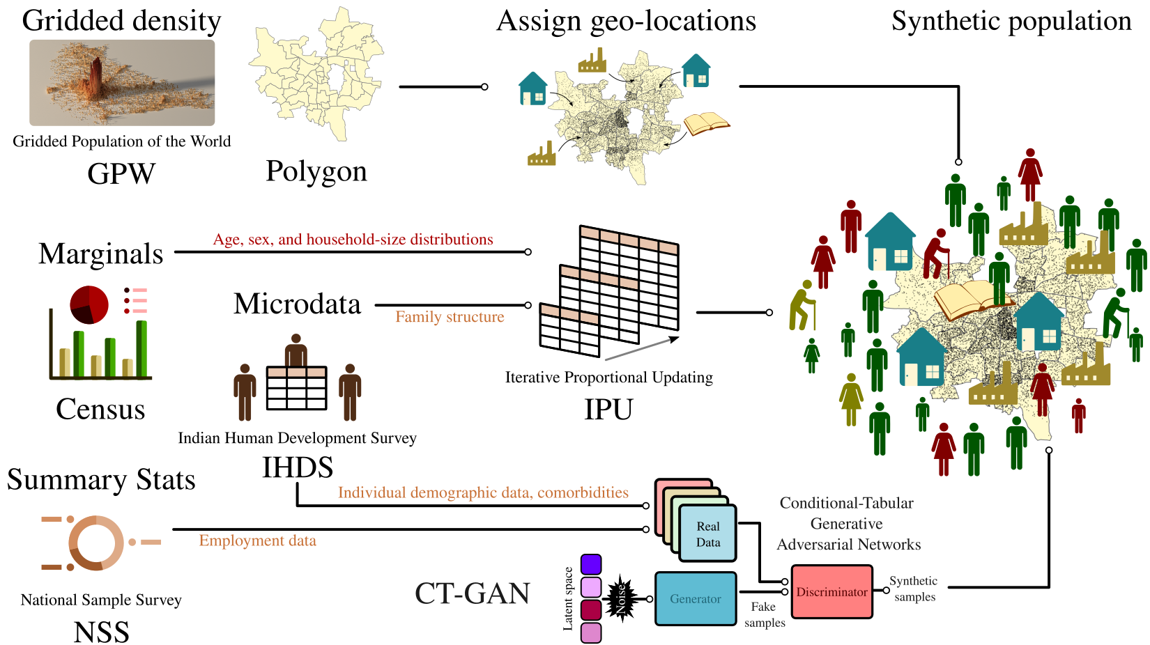
We use a variety of data sources to generate a population of individuals and households with demographic attributes that are statistically identical to real data. This population is generated using statistical methods and machine learning algorithms that are flexible enough to generate data at various administrative levels, ranging from small communities to states. The primary sources of data for these algorithms include the Census of India, the India Human Development Survey (IHDS), the National Sample Survey (NSS), the National Family Health Welfare Survey (NFHS), and the Gridded Population of the World (GPW).
While the synthetic population should faithfully reproduce demographic statistics, it must also incorporate other realistic network structures, such as those appropriate to households and workplaces. (Otherwise, we could end up, for example, with “families” composed entirely of toddlers, or workplaces with strange mixes of professions.) Because different kinds of data respond well to different techniques, a hybrid process is used to scale up these datasets. First, the data is cleaned to remove obvious inconsistencies. Next, a customised hybrid of Iterative Proportional Fitting (IPF), Iterative Proportional Updating (IPU), and a specialised variant of a neural network, called a Conditional-Tabular Generative Adversarial Network (CTGAN), is used to generate new data.
Briefly, Iterative Proportional Fitting finds a joint distribution that matches the marginals, while trying to stay as close to the sample distribution as possible. Iterative Proportional Updating is a heuristic iterative approach which can simultaneously match or fit to multiple distributions (constraints). Finally, Conditional-Tabular Generative Adversarial Networks is a method to model the tabular data distribution and sample rows from the distribution. A Generative Adversarial Network (GAN) uses two “competing” neural networks, the generator and the discriminator. The generator creates realistic samples with the goal that the discriminator should be unable to differentiate between a real sample and a generated sample. In this zero-sum game, capabilities of both the networks are enhanced iteratively.
Critically, our techniques are designed to work seamlessly across data-scarce and data-rich areas; even if a particular area has error-prone or missing data, a synthetic population can still be generated, albeit of a lower quality.
Generating a synthetic population
We use IPF to generate a base population, using census data for the demographics and the IHDS survey dataset for personal and household attributes. The base population thus consists of individual data and household data. We assign each household to an administrative unit within a district.
We also experimented with CTGAN to generate a base population. The major advantage of IPU over CTGAN is that IPU is capable of matching individual level and household level characteristics of an individual while making sure that members of the household have a realistic age and gender joint distribution.
To assign job labels to individuals, the relevant data from the IHDS dataset is used. For the time-being, we classify individuals below the age of 18 as students, but could easily relax this assumption. A subset of the population is also assumed be home-bound. This subset consists of unemployed individuals, homemakers, infants and children under the age 3 and elderly people over the retirement age. We use data from the NSS survey to determine the percentage of adult males and females in a city who are home-bound.
Each student in the population is assigned a school. Similarly, each working individual is assigned a workplace based upon their job label. We generate a synthetic latitude and longitude pair for each home, school and workplace in our dataset using GADM grid population density data.
To assign an individual a school, we sample from the list of schools within that geographical boundary, weighing each school by the inverse of the euclidean distance between it and the individual's home. This weighting factor increases the probability of assigning an individual a school that is closer to their home. We follow a similar method to assign workplaces to adults. Additionally, based on every individual's job label, a workplace is assigned at random from a suitable subset of allowed workplaces.
A number of additional attributes are included in our synthetic population, including whether an individual uses public transport or whether an individual is an essential worker. These values are assigned using the individual's job label.
Verifying the generated population
The figure below compares the marginal distributions of age, height, and weight across samples of the survey and the synthetic population for the combined districts of Mumbai and Mumbai Suburban. We work with a randomly chosen subset comprising 10,000 individuals to compare with the survey data, although our synthetic population has 12 million individuals.
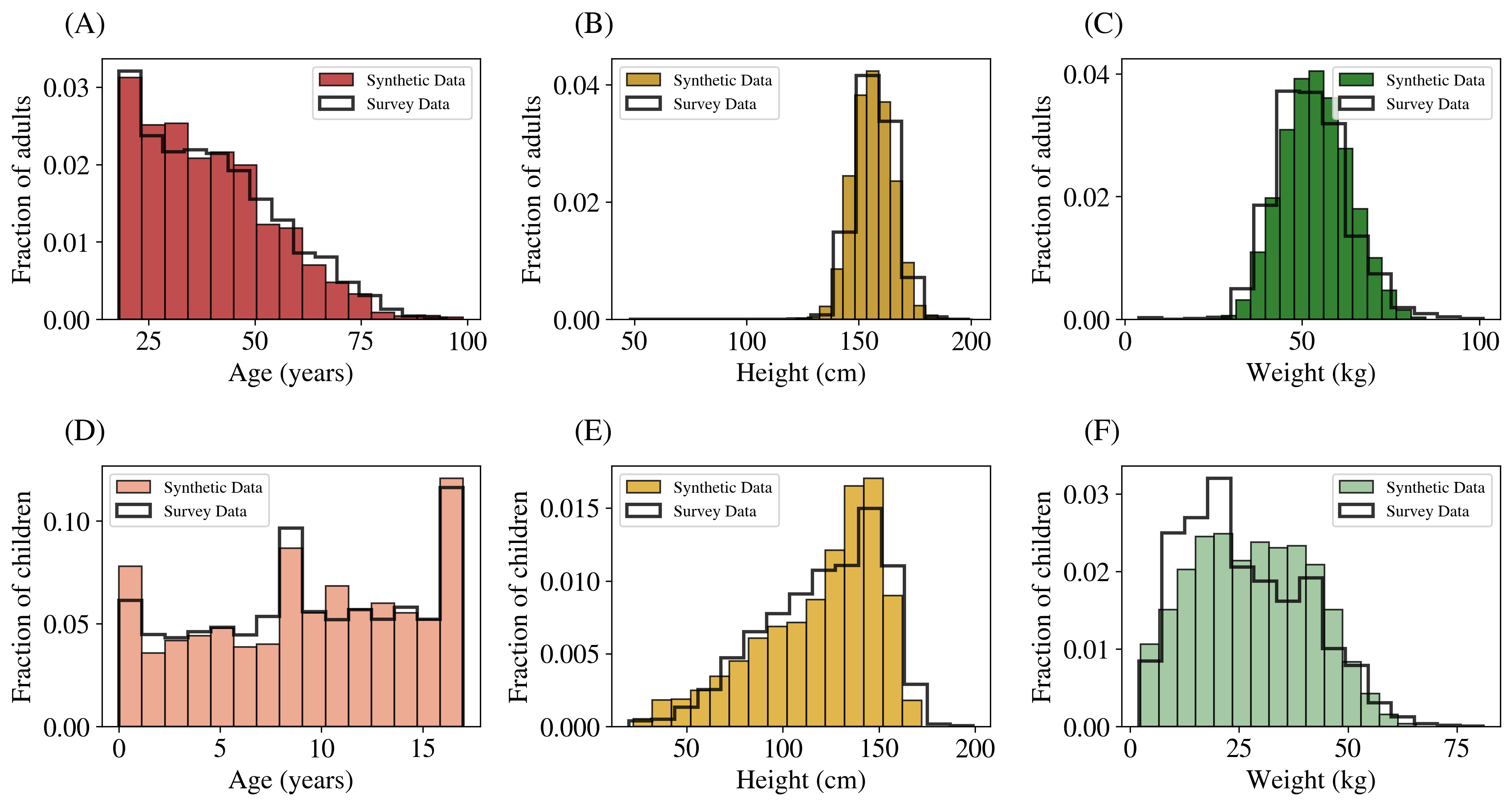
The table below summarises two statistical tests: the two-sample Kolmogorov–Smirnov (KS) test and the Chi-Squared (CS) test. These tests are conducted on compatible columns in both the survey and the synthetic population: the CS test is applied to categorical or Boolean columns (sex in our population), while the KS test is applied to numerical columns (age, height, and weight). For the CS test, the confidence level is the p-value; for the KS test we report 1 − (KS statistic).
| Test | Confidence level |
|---|---|
| CS Test for Sex | 0.99 |
| KS Test for Age | 0.98 |
| KS Test for Height | 0.91 |
| KS Test for Weight | 0.95 |
Critically, our techniques are designed to work seamlessly across data-scarce and data-rich areas; even if a particular area has error-prone or missing data, we can still generate a synthetic population, albeit of slightly poorer quality, but without affecting anything else.